Subtopic Archive - Page 3 of 10

One sided Limits from graphs

December 3, 2019/by admin_ct

How to find limits from graphs

Sometimes it is important to investigate and work on one sided limits because a limit exist only when left and right sided limits exist separately and are same. When we approach to x from lesser values (left side) then it is called left sided limit and when we approach to x from greater values (right side) then it is called Right sided Limit.

At holes left and right sided limits exist and are same but the function is not continuous there.
lets work on some examples where we find limits from the given graph.

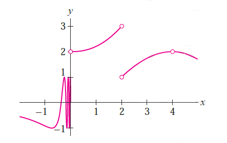
Example1:The function f(x) in given graph is not defined at x=0,2,4. Investigate the one and two sided limits at these points.

Solution: At x=0,

Left hand limit $\dpi{120} \lim_{x\rightarrow 0^{-}}f(x) = DNE$

left side limit at x=0 doesn’t exist because function oscillates infinitely towards left of 0.

Right hand limit $\dpi{120} \lim_{x\rightarrow 0^{+}}f(x) = 2$

since both limits are not same so limit doesn’t exist at x=0

$\dpi{120} \lim_{x\rightarrow 0}f(x) = DNE$

At x= 2

left hand limit $\dpi{120} \lim_{x\rightarrow 2^{-}}f(x) = 3$

Right hand limit $\dpi{120} \lim_{x\rightarrow 2^{+}}f(x) = 1$

Both one sided limits exist separately but not equal so limit does not exist (DNE) at x=2

$\dpi{120} \lim_{x\rightarrow 2}f(x) = DNE$

At x=4

left hand limit $\dpi{120} \lim_{x\rightarrow 4^{-}}f(x) = 2$

Right hand limit $\dpi{120} \lim_{x\rightarrow 4^{+}}f(x) = 2$

Both one sided limits exist at x=4 and are equal , so limit exist at x=4

$\dpi{120} \lim_{x\rightarrow 4}f(x) = 2$

Infinite Limits:

Some functions f(x) tends to +∞ or -∞ when x approach to a value c, then $\dpi{120} \lim_{x\rightarrow c}f(x)$ does not exist and we say f(x) has an infinite limit. One sided limits can be infinite limits. More precisely we write it as,

$\dpi{120} \lim_{x\rightarrow c}f(x) = \infty$

$\dpi{120} \lim_{x\rightarrow c}f(x) = -\infty$

When f(x) approach to ∞ or -∞ from one or both sides then line x=c is called Vertical Asymptote.Limits does not exist at vertical asymptotes.

Here is an example to understand this concept graphically.

Example2: Investigate one sided limits graphically.

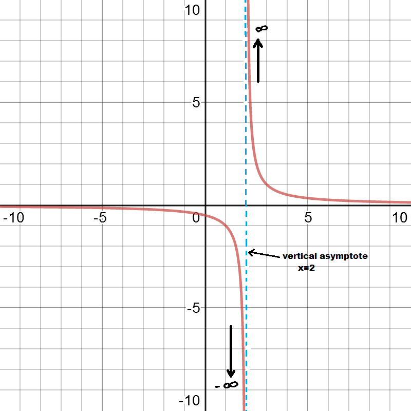
a) $\dpi{120} {\color{Red} \lim_{x\rightarrow 2}\frac{1}{x-2}}$

Observing the graph , we find that y values are approaching to -∞ as we move closer to x=2 from left side and y values are approaching to ∞ as we move closer to x=2 from right side.

$\dpi{120} \lim_{x\rightarrow 2^{-}}\frac{1}{x-2}= -\infty$

$\dpi{120} \lim_{x\rightarrow 2^{+}}\frac{1}{x-2}= \infty$

Both one sided infinite limits are not same. That means limits does not exist at x=2

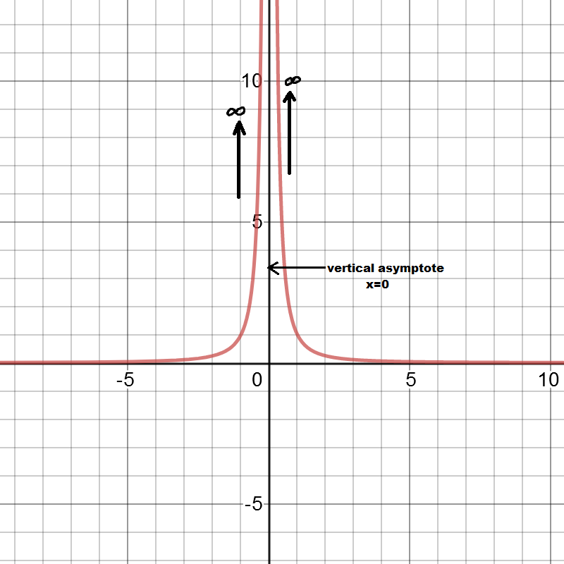
b) $\dpi{120} {\color{Red} \lim_{x\rightarrow 0}\frac{1}{x^{2}}}$

Looking at the graph,we find that y values are approaching to ∞ when we move closer to x=0 from both left and right sides.

That means both one sided infinite limits are same. But infinite limit itself does not exist therefore limit doesn’t exist at x=0

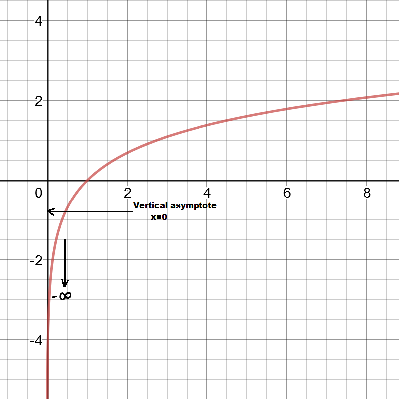
c) $\dpi{120} {\color{Red} \lim_{x\rightarrow 0}ln(x)}$

Natural log (ln) is not defined for negative values so its domain is (0,∞). Looking at the graph we find that y values are approaching to -∞ when we move closer to 0 from right side. Only one right sided limit is possible, which doesn’t exist being infinite limit. So x=0 is a vertical asymptote and limit does not exist here.

Find limits from the given graph.

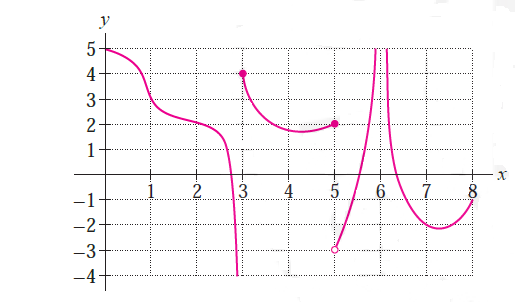
Example3: Determine the one sided limits of the function f(x) at points x=1,3,5,6 in the following graph.

Solution; At x=1

Function is defined and continuous at x=1. Both left and right sided limits approach to same number(3), so limit exist here.

$\dpi{120} \lim_{x\rightarrow 1}f(x)=3$

At x=3

As we move closer to 3 from left , y values approach to -∞ whereas y value is 4 as we move towards 3 from right.

$\dpi{120} \lim_{x\rightarrow 3^{-}}f(x)= -\infty$

$\dpi{120} \lim_{x\rightarrow 3^{+}}f(x)= 4$

At x=5

$\dpi{120} \lim_{x\rightarrow 5^{-}}f(x)= 2$

$\dpi{120} \lim_{x\rightarrow 5^{+}}f(x)= -3$

At x=6

Both left and right sided limits are infinite limits where y values approach to ∞ from both left and right sides of x=6. therefore x=6 is vertical asymptote here.

$\dpi{120} \lim_{x\rightarrow 6^{-}}f(x)= \infty$

$\dpi{120} \lim_{x\rightarrow 6^{+}}f(x)= \infty$

Sketching graphs from given limits

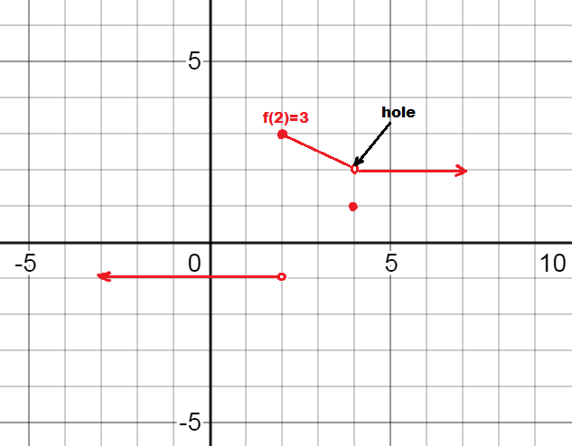
Example 4: Sketch the graph of a function with the given limits.

$\dpi{120} {\color{Red} \lim_{x\rightarrow 2^{+}}f(x)= f(2)=3}$

$\dpi{120} {\color{Red} \lim_{x\rightarrow 2^{-}}f(x)= -1}$

$\dpi{120} {\color{Red} \lim_{x\rightarrow 4}f(x)= 2\neq f(4)}$

Solution:

From first two limits, we conclude that both left and right limits are different when x is approaching to 2. That means graph is approaching to 3 when x values are approaching to 2 from right side. Also function value is 3 at x=2.

Graph is approaching to -1 when x values are approaching to 2 from left.

Limits exist at x=4 and is equal to 2, that means both left and right sided limits are approaching to 2 when x values are approaching to 4 from left and right sides. But function value is not same as limit at x=4 which means there would be a hole at x=4. Gathering all the information above , we get the following graph.

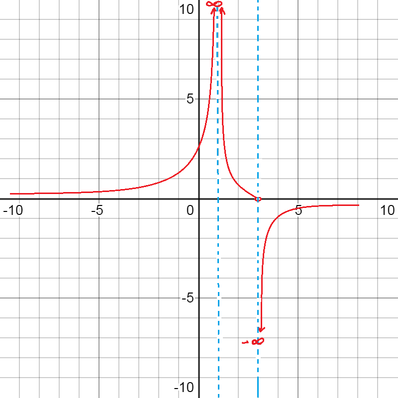
Example 5: Sketch the graph of a function with the given limits.

$\dpi{120} {\color{Red} \lim_{x\rightarrow 1}f(x)= \infty }$

$\dpi{120} {\color{Red} \lim_{x\rightarrow 3 ^{-}}f(x)= 0}$

$\dpi{120} {\color{Red} \lim_{x\rightarrow 3 ^{+}}f(x)= -\infty }$

Solution:

From first limit we note that there is vertical asymptote at x=1 and graph is approaching to infinity from both left and right sides of x=1.

left and right limits are not same at x=3. From left of x=3, graph is approaching to 0 and from right of x=3 graph is approaching to – infinity. Again there is vertical asymptote at x=3.

Converting all the above information into a graph, we get the following graph.

Practice problems:

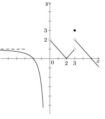
Use the given graph of function to answer each question.

a) $\dpi{120} \lim_{x\rightarrow 0^{-}}f(x)$ b) $\dpi{120} \lim_{x\rightarrow 3 ^{-}}f(x)$ c) $\dpi{120} \lim_{x\rightarrow 3 }f(x)$ d) f(3)= ?

e) $\dpi{120} \lim_{x\rightarrow 0^{+}}f(x)$ f) $\dpi{120} \lim_{x\rightarrow 3 ^{+}}f(x)$ g) $\dpi{120} \lim_{x\rightarrow 0 }f(x)$ h) f(0) = ?

2. Sketch the graph of a function with the following limits.

$\dpi{120} \lim_{x\rightarrow 3^{-}}f(x)=0$

$\dpi{120} \lim_{x\rightarrow 3^{+}}f(x)=4$

$\dpi{120} \lim_{x\rightarrow 1}f(x)=2$

Answers:

1. a) -∞ b) 1 c) DNE d) 3 e) 2 f) 2 g) DNE h) DNE

Graphing linear equation using Slope and Y Intercept

November 30, 2019/by admin_ct

How to graph a line using slope and y intercept.

To graph a line using slope and y intercept , we should have the equation in slope intercept form(y=mx+b) . So we have to convert the linear equation in slope intercept form , if not given already.

Slope Intercept form: y=mx+b

Here coefficient of x is slope(m) and constant term b is y intercept.

Steps to graph using slope and y intercept:

1. Identify y intercept (b) from given equation which can be written as (o,b) in ordered pair form. This gives you first point on y axis.

2. Identify slope(m). Positive slope gives you rising line and negative slope gives you falling line.

$\dpi{120} \mathbf{Slope(m)= \frac{y}{x}=\frac{Rise}{Run}}$

Numerator of slope tells you how many steps you need to move up or down whereas denominator tells us how many steps to need to move left or right.

For positive slope we always go up (rise) , for negative slope we always go down.

3. Right direction of slope takes you to the second point. Joining these two points gives to graph of linear equation.

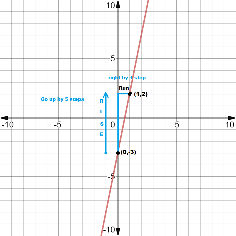
Example1: Find slope and y intercept of equation y = 5x-3 and then graph the equation.

Solution: Comparing the given equation with slope intercept form y=mx+b, we get

Slope(m)=5

Y intercept (b)=-3

Rewriting y intercept in ordered pair form , we get first point as (0,-3) which is always on y axis.

$\dpi{120} Slope(m)=\frac{Rise}{Run}=\frac{5}{1}$

From first point rise 5 steps and then run 1 step right.The point where we stop at, is the second point. Join these two points and get the graph of line equation.

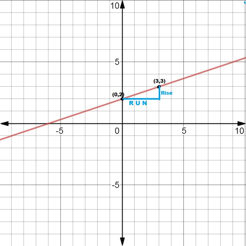
Example2: Find slope and y intercept of equation 3y-x=6 and then graph it.

Solution: Since this equation is not in slope intercept form, so we convert it in that form first.

3y-x =6

3y =x+6

$\dpi{120} y=\frac{1}{3}x+\frac{6}{3}$

$\dpi{120} y=\frac{1}{3}x+2$

Comparing it with y=mx+b, we get y intercept (0,2) as first point on y axis.

$\dpi{120} Slope(m)=\frac{Rise}{Run}=\frac{1}{3}$

From first point rise 1 step and run 3 steps right. We reach at second point (3,3). Join these two points and get the graph of given line equation.

We can also first run by 3 steps right and then rise by one step reaching at the same point

Example3:Find slope and y intercept of the given equation and then graph the equation.

$\dpi{120} {\color{Red} y=\frac{-5}{4}x +1}$

Solution: Comparing the given equation with y=mx+b we get,

Slope(m)=-5/4

Y intercept = (0,1)

$\dpi{120} Slope(m)=\frac{Rise}{Run}=\frac{-5}{4}$

First plot y intercept (0,1) as first point on y axis. Since slope is negative so we go down by 5 steps instead of going up. Basically we should say Fall instead of Rise. After going down by 5 steps , move right by 4 steps and we reach at second point (4,-4).

Join these two points and get the following graph.

Practice problems:

Find slope and y intercept of the given equation and then graph the equation y=2x+3
Convert the given equation in slope intercept form. Find slope and y intercept and then graph the equation 3x-6y=9
Find slope and y intercept of the given equation and then graph the equation y= -2x/3 +1

Graphing linear equations in two variables

November 25, 2019/by admin_ct

Graph linear equations by plotting points

Any linear equation in two variables, x and y is called linear equation in two variables and its graph is drawn on a two dimensional plane. If linear equation is not in explicit form then we convert it by isolating y, step by step.

Steps to draw graph of linear equation:

1. Isolate y, if the equation is not given in explicit form.

The equation where y is written all by itself i.e y=mx+b, is called explicit form of equation, whereas Ax+By+c=0 is called implicit form of linear function.

2. Make a table with two rows, first row labeled as x and other row labeled as y.

3. Select some random values of x.These values should be selected in such a way that we don’t get very large values of y. We should get y values without much effort and should be free of fractions.Keeping that in mind using one value as x=0 always help.

4. Plugin those x values into the given equation in explicit form and solve for y.

5.Write these x and y values as points in ordered form. Three points are good enough to get a beautiful graph .

6. Plot these points on a suitable grid and join the points by a line. If all points doesn’t lie on same line then check the work for that point there may be some mistake.

Lets work on some examples to understand the process.

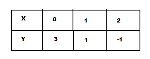
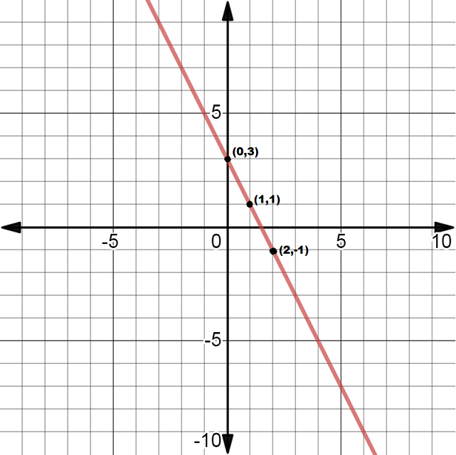
Example1: Graph the equation y=-2x+3 by plotting points.

Solution: Since this equation is already in explicit form so we start getting table of x,y values. lets use x=0,1,2 as random x values. You can also use -1,0,1 . Plugin those x values into the given equation and get y values.

For x=0, y=-2(0)+3 = 3 (0,3)

For x=1, y=-2(1)+3 =1 (1,1)

For x=2, y=-2(2)+3=-1 (2,-1)

Now plot all these points on a grid and join these points to get following line graph.

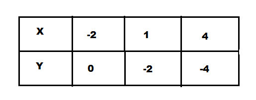
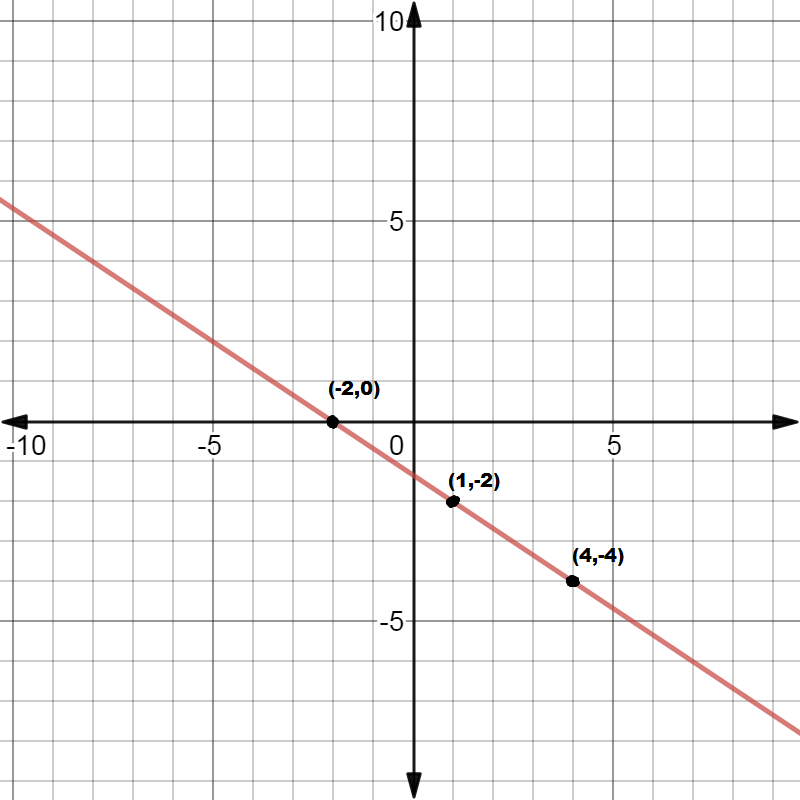
Example2: Graph the equation 2x+3y+4=0 by plotting points.

Solution: First we get this equation in explicit form. For that we get y by itself step by step.

3y=-2x-4

$\dpi{120} y=\frac{-2}{3}x -\frac{4}{3}$

Next we get a table of x,y values in order to get the points. We should select such x values which doesn’t result in fractional y values. Initially you will find some difficulty in finding such values but after some practice you would be able to do all that math in your mind.

For x=-2, y= -2(-2)/3 – 4/3 = 4/3 -4/3 =0 (-2,0)

For x=1, y= -2/3 -4/3 = -6/3 = -2 (1,-2)

For x=4, y=-2(4)/3 -4/3 = -8/3 – 4/3=-12/3=-4 (4,-4)

Plotting all these three points on a grid and joining them we get following graph.

Graph Linear equations by finding Intercepts

Graph of a linear equation can be drawn using x and y intercepts instead of plotting random points.

X intercept : This is the point where graph intersect the x axis. To get x intercept , always plugin y=0 and solve for x. X intercept is written in the form (x,0)

Y intercept: This is the point where graph intersect the y axis. To get y intercept , always plugin x=0 and solve for y. Y intercept is written in the form (0,y)

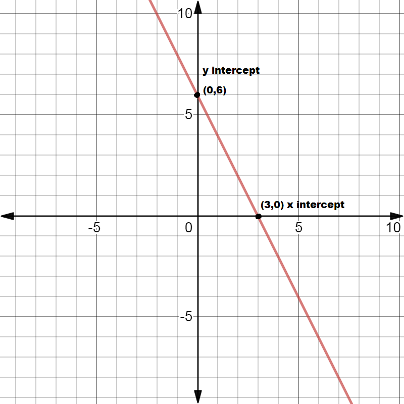
Example3: Find the intercepts of y= -2x+6 and then graph the equation using intercepts only.

Solution;

X intercept: Plugin y=0 and solve for x.

0=-2x+6

-6=-2x

3=x => (3,0)

Y intercept: Plugin x=0 and solve for y.

y= -2(0)+6

y=6 => (0,6)

When we plot these two points on a grid, we get the following graph.

Practice problems:

Find at least three random points for equation y=5x-4 and graph the equation by plotting those points.
Graph the equation 5y-x=10 by plotting points. Be sure to get integers for your points not decimals.
Find x and y intercepts for 3x+2y=6. Graph the equation using these intercepts.

Answers:

(0,-4) , (1,1), (2,6)
(-5,1) , (0,2), (5,3)
X intercept (2,0) Y intercept (0,3)

Cartesian coordinate system

November 24, 2019/by admin_ct

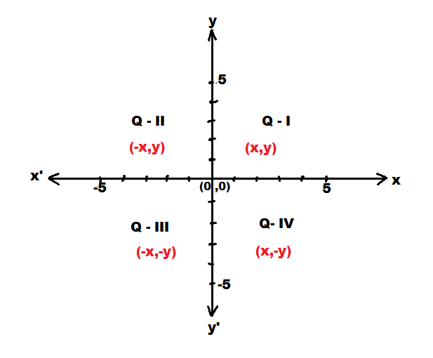
The Cartesian coordinate system , also called rectangular system consists of two dimensional plane (x,y Plane). This two dimensional plane is divided into 4 quadrants by X axis(horizontal axis) and Y axis (vertical axis).

The point where both axes intersect each other, is called origin (0,0). Towards the right and above of origin there are increasing positive numbers. Towards the left and down of origin there are decreasing negative numbers. Each axis extend to positive and negative infinity represented by arrowheads.

Each point in this plane is represented by ordered pair (x,y). First one is x coordinate which represents the horizontal distance of point from the origin and latter one is y coordinate which represents the vertical distance of point from origin.

If the point is of the form (x,0) i.e when y coordinate is 0 then point always lie on x axis.

If the point is of the form (0,y) i.e when x coordinate is 0 then point always lie on y axis.

In 1st quadrant both x and y are positive, so any point in this quadrant is represented as (x,y).

In 2nd quadrant x is negative and y is positive , so any point in this quadrant is represented as (-x,y).

In 3rd quadrant both x and y are negative, so any point in this quadrant is represented as (-x,-y).

In 4th quadrant x is positive but y is negative, so any point in this quadrant is represented as (x,-y)

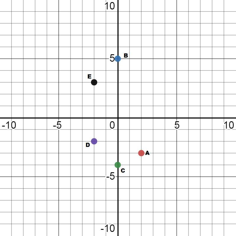
Example: Plot the following points on the x-y plane .

A(2,-3), B(0,5), C(0,-4), D(-2,-2), E(-2,3)

Solution:

Related Rates

November 15, 2019/by admin_ct

Derivative as a Rate measure

Let y=f(x) be a function of x. Let Δy be the change in y corresponding to a small change in x. Then Δy/Δx represents the change in y due to a unit change in x. Δy/Δx represents the average rate of change of y with respect to x. As Δx →0 , this average rate of change becomes the instant rate of change.

Instant rate of change $\lim_{\Delta x \to 0 }\frac{\Delta y}{\Delta x}=\frac{dy}{dx}$

Instant word is often dropped and dy/dx represents the rate of change of y with respect to x.

If the y value changes with respect to time (t) then rate of change in y is represented as dy/dt.

Lets take an example of balloon which is being filled with air , so its volume and radius both are changing with respect to time. We represent them as dv/dt and dr/dt. These are called related rates because volume V is related to radius r.

Example1: Find the rate of change of the area of a circle with respect to its radius . How fast the area changing with respect to radius when radius is 3 cm?

Solution: let A be the area of circle

A=πr^2

To find rate of change of area with respect to radius, we need to find dA/dr.

dA/dr =π*2r = 2πr

When r=3 then rate of change of area is given as,

dA/dr= 2π*3= 6π cm^2/cm

Example2: Find the rate of change of volume of a sphere with respect to its surface area when its radius is 2 cm.

Solution: Volume of sphere $V= \frac{4}{3}\pi r^{3}$

$\frac{dV}{dr}=\frac{4}{3}*3\pi r^{2}= 4\pi r^{2}$

Surface area of sphere $A=4\pi r^{2}$

$\frac{dA}{dr}= 4\pi *2r= 8\pi r$

We need to find rate of change of volume V with respect to surface area A

$\frac{dV}{dA}=\frac{\frac{dv}{dr}}{\frac{dA}{dr}}=\frac{4\pi r^{2}}{8\pi r}=\frac{r}{2}$

We need to find rate of change when r=2 so plugin r=2

$\frac{dV}{dA}=\frac{2}{2}=1$ cm.

Steps to solve related rate problem

Sketching diagram for ongoing situation always helps and label it with variables.
Express the given information mathematically and mention the quantity(variable) to be found.
Write an equation/expression showing the relation between different variables.
Find the derivative and solve for the asked quantity/variable.
If required find the remaining variables at that instant.

Possible relations used in related rates problems:

1. Pythagorean Theorem:

$\dpi{120} \mathbf{x^{2}+y^{2}=z^{2}}$

2. Trigonometric relations like,

y= x tanθ , y=z sinθ , x= z cosθ

3. Similar triangles

y/b = x/a or y/x = b/a

4. Area and volume formulas

Rectangle area = xy , Circle area = πr^2

surface area of sphere= 4πr^2 , volume of cone = 1/3*πr^2h

volume of sphere= 4/3*πr^3, volume of cube = x^3

lets work on some examples to understand the process better.

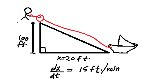
Example3. A boat is pulled on shore by rope from a 20 feet high quay wall. If the rope is pulled at a rate of 15 ft/min, at what rate is the boat approaching the shore when it is 100 ft away from the shore?

Solution:

Given: dz/dt = -15 ft/min and y=20 ft.

To find: dx/dt when x=100 ft.

There is Pythagorean relation between all three quantities.

$\dpi{120} \mathbf{x^{2}+y^{2}=z^{2}}$

Differentiating both sides with respect to time(t) to find rate of change,

$\dpi{120} 2x\frac{dx}{dt}+ 0=2z\frac{dz}{dt}$ [derivative of y^2 is 0 since wall height y, is a constant]

$\dpi{120} \frac{dx}{dt}=\frac{z}{x}\frac{dz}{dt}$

Here, we also need to find value of z using Pythagorean theorem,

$\dpi{120} (100)^{2}+(20)^{2}=z^{2}$

$\dpi{120} z=\sqrt{10400}= \sqrt{400*26}=20\sqrt{26}$

Using this z value and other given values, we can rewrite the equation as

$\dpi{120} \frac{dx}{dt}=\frac{20\sqrt{26}}{100}*(-15)$

$\dpi{120} \frac{dx}{dt}=-3\sqrt{26}$ ft/min

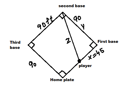
Example4:Recall that in baseball the home plate and the three bases form a square of side length 90 ft. A batter hits the ball and
runs to the first base at 24 ft/sec. At what rate is his distance from the 2nd base decreasing when he is halfway to the first base.
Solution:

Let distance between player and first base=x
let distance between player and 2nd base =z
Given: dx/dt = -24 ft/sec
Find: dz/dt when x = 90/2 = 45 ft.

There is Pythagorean relation between all three quantities.

$\dpi{120} z^{2}=x^{2}+(90)^{2}$

$\dpi{120} 2z\frac{dz}{dt}=2x\frac{dx}{dt}+0$

$\dpi{120} \frac{dz}{dt}=\frac{x}{z}\frac{dx}{dt}$

Here, we also need to find z to find dz/dt

$\dpi{120} z =\sqrt{(45)^{2}+(90)^{2}} = \sqrt{10125}$ $\dpi{120} z =\sqrt{(45)^{2}+(90)^{2}} = \sqrt{10125}=45\sqrt{5}$

Using these values of z= 25√5 , x= 45

$\dpi{120} \frac{dz}{dt}=\frac{x}{z}\frac{dx}{dt}$

$\dpi{120} \frac{dz}{dt}=\frac{45}{45\sqrt{5}}(-24) =\frac{-24}{\sqrt{5}}$ ft/sec

So the distance between player and second base is decreasing at the rate of 24/√5 ft/sec.

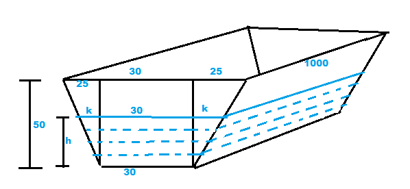
Example5 :A water trough is 10 m long and a cross-section has the shape of an isosceles trapezoid that is 30 cm wide at the bottom, 80 cm wide at the top, and has height 50 cm. If the trough is being filled with water at the rate of 0.2 m^3/min, how fast is the
water level rising when the water is 30 cm deep?

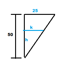
Solution: Firstly, lets draw the diagram for this situation and label it.

Given : length of trough =10m =1000cm , height of trough = 50 cm

Lower base =30 cm, upper base = 80 cm

dv/dt=0.2m^3/min = 200000 cm^3/min

To find = dh/dt (rate of change of water level)

Here we use similar triangles theorem ,

$\dpi{120} \frac{25}{k}=\frac{50}{h}$

$\dpi{120} \frac{1}{k}=\frac{2}{h}\Rightarrow h=2k$

We know that volume of water = Trapezoid area * height

V= [1/2(lower base+ upper base)length] * height

V= 1/2(30+ 30+2k)1000*h

V= (60+2k)500h

V=(60+h)500h

V=30,000h+500h^2

Taking derivative of both sides,

$\dpi{120} \frac{dV}{dt}=30,000 \frac{dh}{dt}+1000h*\frac{dh}{dt}$

$\dpi{120} 200000=30,000 \frac{dh}{dt}+1000(30)*\frac{dh}{dt}$

$\dpi{120} 200000=60,000 \frac{dh}{dt}$

$\dpi{120} \frac{200000}{60000}= \frac{dh}{dt}$

10/3 = dh/dt

So the water level is rising at the rate of 10/3 cm/min

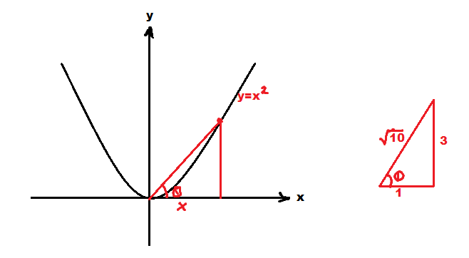
Example6. A particle is moving along the graph of y = x^2 in such a way that its x-coordinate is increasing at a constant rate of 10 units per second. Let θ be the angle between the positive x-axis and the line joining the particle to the origin. Find the rate at
which θ is changing when the x-coordinate of the point is 3.

Solution:

Given: x=3 and dx/dt = 10 units/sec

To find : dθ/dt

Using the relationship in right triangle we get,

$\dpi{120} tan\theta =\frac{y}{x}$

$\dpi{120} tan\theta =\frac{x^{2}}{x}\Rightarrow tan\theta =x$

x=tanθ

Taking derivative of both sides,

$\dpi{120} \frac{dx}{dt}=sec^{2}\theta \frac{d\theta }{dt}$

$\dpi{120} cos^{2}\theta \frac{dx}{dt}=\frac{d\theta }{dt}$ ———- (i)

In the right triangle we also need to find angle θ and hence cosθ when x=3

we have $\dpi{120} tan\theta =\frac{y}{x}=\frac{3}{1}$

Using Pythagorean we get hypotenuse as √(3^2 +1^2) = √10

so cosθ=1/√10

Using value of cosθ in equation (i)

$\dpi{120} \left ( \frac{1}{\sqrt{10}} \right )^{2}*10=\frac{d\theta }{dt}$

$\dpi{120} \frac{10}{10}=\frac{d\theta }{dt}$

$\dpi{120} 1 =\frac{d\theta }{dt}$

So angle θ is changing at the rate of 1 rad/sec

Practice problems:

1. The width of a rectangle is increasing at a rate of 3 cm/s while its height is decreasing at a rate of 4 cm/s. Find the rate at which the area of the rectangle is changing when the width is 12 cm and the height is 20 cm.

2. A man 2 m high walks at a uniform speed of 5km/hr away from a lamp post which is 6m high.Find the rate at which length of his shadow increases.

3.Sand is being poured onto a conical pile at a constant rate of 50 cm^3/min such that height of the cone is always one half of the radius of its base. How fast is the height of pile increasing when sand is 5cm deep.

4.A circular oil slick of uniform thickness is caused by a spill of 1 m^3 of oil. The thickness of the oil slick is decreasing at a rate of 0.1 cm/hr. At what rate is the radius of the slick increasing when it is 8 m?

Answers:

12 cm^2/sec
2.5 km/hr
1/2π cm/min
0.256π m/hr

Linear Approximation and Linearization

November 9, 2019/by admin_ct

Linear approximation

Let Δx be a small change in x , then Δf is the corresponding change in y value which is given as…

Δf=f(a+Δx)-f(a)

lets use derivative to compute this small change Δf, without computing it directly.

By the definition of derivative,

$\dpi{120} f'(a)=\lim_{\bigtriangleup x->0}\frac{f(a+\bigtriangleup x)-f(a)}{\bigtriangleup x}=\lim_{\bigtriangleup x\rightarrow 0}\frac{\bigtriangleup f}{\bigtriangleup x}$

When Δx is very small, we have

$\dpi{120} \mathbf{\frac{\bigtriangleup f}{\bigtriangleup x}=f'(a)}$

Δf=f ‘(a)Δx This is the formula for linear approximation.

Example1: Use equation $\dpi{120} {\color{Red} \frac{\bigtriangleup f}{\bigtriangleup x}=f'(a)}$ to estimate Δf= f(3.02)-f(3) for f(x)= tan(πx/3).

Solution: Here we have a=3 , Δx= 0.02 and f(x)= tan(πx/3)

Δf=f(3.02)-f(3)

$\dpi{120} f'(x)=sec^{2}\left ( \frac{\pi x}{3} \right )*\frac{\pi }{3}$

$\dpi{120} f'(3)=sec^{2}\left ( \frac{\pi 3}{3} \right )*\frac{\pi }{3}$

$\dpi{120} f'(3)=sec^{2}\left (\pi \right )*\frac{\pi }{3}=(-1)^{2}*\frac{\pi }{3}=\frac{\pi }{3}$

Using formula $\dpi{120} \frac{\bigtriangleup f}{\bigtriangleup x}=f'(a)$ we have Δf= f ‘(a)Δx

Δf = f ‘(3)Δx = π/3(0.02) = 0.02094

Differential Notation:

Linear approximation can also be written using differentials dx and dy, In that case dx is used in place of Δx and dy is used in place of Δf and the expression becomes,

dy = f ‘(a)dx

This is simply another way of writing Δf=f ‘(a) Δx

Example2. Estimate the following using differentials.

$\dpi{120} {\color{Red} ln(e^{3+0.1})-ln(e^{3})}$

Solution: First we need to recognize the function f(x) here which is ln(e^x)

f(x)=ln(e^x) which can be simplified to,

f(x)= x lne = x

f ‘(x)= 1

here we have a=3 and dx= 0.1

so dy = f ‘(a)dx = 1(0.1)= 0.1

Example3.Estimate Δy using differentials.

$\dpi{120} {\color{Red} y=\frac{10-x^{2}}{2+x^{2}} , a=1, dx=0.01}$

Solution:

$\dpi{120} f(x)=\frac{10-x^{2}}{2+x^{2}}$

$\dpi{120} f'(x)=\frac{(2+x^{2})(10-x^{2})'-(2+x^{2})'(10-x^{2})}{(2+x^{2})^{2}}$

$\dpi{120} f'(x)=\frac{(2+x^{2})(-2x)-(2x)(10-x^{2})}{(2+x^{2})^{2}}$

$\dpi{120} f'(x)=\frac{-24x}{(2+x^{2})^2}$

$\dpi{120} f'(a)=\frac{-24(1))}{(2+1^{2})^2}= \frac{-8}{3}$

Using differentials,

dy= f ‘(a) dx

dy =(-8/3)(0.01) = -0.02667

Linearization:

We use linearization to approximate the function itself rather than the change Δf. If a function is differentiable at x=a and x is close to a then function is approximated by linearization L(x) given as,

L(x)=f ‘(a)(x-a)+f(a)

Note:Linearization and linear approximation are the two ways of saying same thing !

Example4: Estimate using linear approximation and find the error using calculator.

$\dpi{120} {\color{Red} \frac{1}{\sqrt{101}}-\frac{1}{10}}$

Solution: Here we have f(x)=1/√x and a=100 , Δx=101-100=1

$\dpi{120} f'(x)= \frac{-1}{2}x^{\frac{-3}{2}}=\frac{-1}{2x^{\frac{3}{2}}}$

$\dpi{120} f'(a)=\frac{-1}{2(100)^{\frac{3}{2}}}=\frac{-1}{2(10)^{3}}=\frac{-1}{2000}$

Δf = f ‘(a) Δx

$\dpi{120} \Delta f=\frac{-1}{2000}(1)= -0.0005$

Calculator value $\dpi{120} \frac{1}{\sqrt{101}}-\frac{1}{10}= -4.96280\times 10^{-4}$

Error ≈|-4.96280*10^-4 -(-0.0005)| =3.7190*10^-6

Percentage error :

Percentage error $\dpi{120} = \left |\frac{error}{actual value} \right |*100$

Example5: The atmospheric pressure at altitude h (kilometers) for 11 ≤ h ≤25 is approximately
$\dpi{120} {\color{Red} p(h)= 128e^{-0.157h}}$ kilopascals
(a) EstimateΔ P at h = 20 when Δh = 0.5.
(b) Compute the actual change, and compute the percentage error in the Linear Approximation.

Solution; (a)

Using formula Δp=p'(a)Δh , first we find derivative p'(a) at a=20

$\dpi{120} p'(h)= 128e^{-0.157h}*(-0.157)= -20.096e^{-0.157h}$

$\dpi{120} p'(20)= -20.096e^{-0.157*20}= 20.096*(0.043282)= -0.8698111$

Plugin value of p'(20) into formula we get,

Δp=-0.869811*0.5 = -0.434906 kilopascals

(b) Actual change p(20.5)- p(20)=128(0.040015-0.043282)= -0.418278 kilopascals

error = |-0.434906-(-0.418278)| = 0.016628

Percentage error = $\dpi{120} \left |\frac{0.016628}{0.418278} \right |*100 = 3.975$

So percentage error is 3.98%

Example6: Find linear approximation function to estimate √0.037 and then estimate it.

Solution:First we recognize the function as f(x)=√x

which is close to perfect square 0.04, so here we have a=0.04 .

$f'(x)= \frac{1}{2}x^{\frac{-1}{2}}=\frac{1}{2\sqrt{x}}$

$f'(a)= \frac{1}{2\sqrt{0.04}}=\frac{1}{2(0.2)}=\frac{1}{0.4}$

Also f(a)= √0.04 = 0.2

Linear approximation is given as,

L(x)=f ‘(a)(x-a)+f(a)

$L(x)= \frac{1}{0.4}(x-0.04)+ 0.2$

To estimate √0.037 we plugin x as 0.037 in the linear approximation formula found above.

$L(x)= \frac{1}{0.4}(x-0.04)+ 0.2$

$L(0.037)= \frac{1}{0.4}(0.037-0.04)+ 0.2 = \frac{-0.003}{0.4}+0.2$

$L(0.037)= 0.2-\frac{3}{400}=0.2-0.0075 =0.1925$

Practice problems:

Which is larger √2.1-√2 or √9.1 – √9. Explain using linear approximation.
Estimate Δf. Using calculator , compute both error and percentage error. f(x)=√(1+x) , a=3 , Δx=0.2
Estimate Δy using differentials for f(x)= cosx at a=π/6 and dx= 0.014
A thin silver wire has length L = 18 cm when the temperature is T = 30◦C. Estimate ΔL when T decreases to 25◦C if the coefficient of thermal expansion is $k=1.9\times 10^{-5}^{\circ}C^{-1}$

Root Test

November 5, 2019/by admin_ct

How to use Root test.

When series contain powers in terms of n, then we use Root test to get rid of power n or to make powers more meaningful and working. This test is also used to check absolute convergence of series.

This test says if :

i) $\dpi{120} \mathbf{\lim_{n \to \infty }\left | a_{n} \right |^{\frac{1}{n}}<1}$ Then series is convergent .

ii) $\dpi{120} \mathbf{\lim_{n \to \infty }\left | a_{n} \right |^{\frac{1}{n}}>1}$ or ∞ Then series is divergent .

iii) $\dpi{120} \mathbf{\lim_{n \to \infty }\left | a_{n} \right |^{\frac{1}{n}}=1}$ then Root test is inconclusive and use another test.

Examples: Check whether the given series are convergent or divergent.

1) $\dpi{120} {\color{Red} \sum_{n \to 1}^{\infty }\frac{n^{n}}{3^{1+3n}}}$

Here we have $\dpi{120} a_{n}=\frac{n^{n}}{3^{1+3n}}$

So , $\dpi{120} \lim_{n \to \infty }\left | a_{n} \right |^{\frac{1}{n}}= \lim_{n \to \infty }\left | \frac{n^{n}}{3^{1+3n}} \right |^{\frac{1}{n}}$

$\dpi{120} \lim_{n \to \infty }\left | \frac{n^{\frac{n}{n}}}{3^{\frac{1+3n}{n}}} \right |$

$\dpi{120} \lim_{n \to \infty }\left | \frac{n^{1}}{3^{\frac{1}{n}}*3^\frac{3n}{n}} \right |$

$\dpi{120} \lim_{n \to \infty }\left | \frac{n}{3^{\frac{1}{n}}*3^{3}} \right |$

$\dpi{120} \frac{1}{3^{3}}\lim_{n \to\infty }\frac{n}{3^{\frac{1}{n}}}$

$\dpi{120} \frac{1}{27}\frac{\infty }{3^{0}}=\frac{1}{27}\frac{\infty }{1}=\frac{\infty }{27}=\infty$

Since limit is ∞ so this series is divergent !

2) $\dpi{120} {\color{Red} \sum_{n =0}^{\infty }\left (\frac{5n-3n^{3}}{7n^3+2} \right )^{n}}$

Here we have $\dpi{120} a_{n}= \left (\frac{5n-3n^3}{7n^3+2} \right )^{n}$

So, $\dpi{120} \lim_{n \to \infty }\left | a_{n} \right |^{\frac{1}{n}}= \lim_{n \to \infty }\left | \left (\frac{5n-3n^3}{7n^3+2} \right )^{n} \right |^{\frac{1}{n}}$

$\dpi{120} \lim_{n \to \infty }\left | \frac{5n-3n^3}{7n^3 +2} \right |^{\frac{n}{n}}$

$\dpi{120} \lim_{n \to \infty }\left | \frac{-3n^3+5n}{7n^3 +2} \right |^{1}$

$\dpi{120} \left |\lim_{n \to \infty } \frac{-3n^3+5n}{7n^3 +2} \right |$

$\dpi{120} \left | \frac{-3}{7} \right |=\frac{3}{7}<1$

Limit is less than 1 so this series is convergent !

Practice problems:

Check the convergence of following series using root test:

$\dpi{120} \sum_{n=3}^{\infty }\frac{(-12)^{n}}{n}$

2) $\dpi{120} \sum_{n=0}^{\infty }\frac{2^{n}}{3^{n}}$

3) $\dpi{120} \sum_{n=0}^{\infty }\frac{4^{n}}{3^{n+2}}$

Answers:

1) divergent

2) convergent

3) divergent

Ratio Test

October 26, 2019/by admin_ct

How to use ratio test

Whenever we see factorials in series expression then surely we need to use Ratio test. This test can also be used to prove absolute convergence.

This test says :

Suppose we have the series $\dpi{120} \mathbf{\sum_{n=1}^{\infty }a_{n}}$ . Find the ratio of n+1th term to the nth term and find its limit. Follow these rules:

i) if $\dpi{120} \mathbf{\lim_{n \to \infty }\left | \frac{a_{n+1}}{a_{n}} \right |<1}$ Then series is convergent.

ii) if $\dpi{120} \mathbf{\lim_{n \to \infty }\left | \frac{a_{n+1}}{a_{n}} \right |>1}$ or ∞ Then series is divergent.

iii) if $\dpi{120} \mathbf{\lim_{n \to \infty }\left | \frac{a_{n+1}}{a_{n}} \right |=1}$ Then test is inconclusive and use another test.

Examples:

Check the convergence of following series.

1. $\dpi{120} {\color{Red} \sum_{n=1}^{\infty }e^{-n}n!}$

Here we have $\dpi{120} a_{n}= e^{-n}n!$

So $\dpi{120} a_{n+1}= e^{-(n+1)}(n+1)!$

Then,

$\dpi{120} \lim_{n \to \infty }\left | \frac{a_{n+1}}{a_{n}} \right |= \lim_{n \to \infty }\left | \frac{e^{-(n+1)}(n+1)!}{e^{-n}n!} \right |$

$\dpi{120} \lim_{n \to \infty }\left | \frac{e^{-n-1}(n+1)n!}{e^{-n}n!} \right |$

$\dpi{120} \lim_{n \to \infty }\left | \frac{e^{-n}e^{-1}(n+1)}{e^{-n}} \right |$

$\dpi{120} e^{-1} \lim_{n \to \infty }\left | n+1 \right | = \frac{\infty }{e}=\infty$

So this series is divergent !

2) $\dpi{120} {\color{Red} \sum_{n=1}^{\infty }\frac{(n!)^{2}}{(2n)!}}$

Here we have $\dpi{120} a_{n}= \frac{(n!)^{2}}{(2n)!}$

so $\dpi{120} a_{n}= \frac{((n+1)!)^{2}}{(2(n+1))!}= \frac{(n+1)^{2}(n!)^{2}}{(2n+2)!}$

Then $\dpi{120} \lim_{n \to \infty }\left | \frac{a_{n+1}}{a_{n}} \right |= \lim_{n \to \infty }\left | \frac{(n+1)^{2}(n!)^2}{(2n+2)(2n+1)(2n)!}\frac{(2n)!}{(n!)^{2}} \right |$

$\dpi{120} \lim_{n \to \infty }\left | \frac{(n+1)^2}{(2n+2)(2n+1)} \right |$

$\dpi{120} \lim_{n \to \infty }\left | \frac{(n+1)(n+1)}{2(n+1)(2n+1)} \right |$

$\dpi{120} \lim_{n \to \infty }\left | \frac{(n+1)}{2(2n+1)} \right |$

$\dpi{120} \frac{1}{2}\lim_{n \to \infty }\left | \frac{(n+1)}{(2n+1)} \right |$

$\dpi{120} \frac{1}{2}*\frac{1}{2}=\frac{1}{4}$

Since limit is < 1 so this series is convergent !

3) $\dpi{120} {\color{Red} \sum_{n=1}^{\infty }\frac{(2n+1)!}{(n!)^{2}}}$

Here we have $\dpi{120} a_{n}= \frac{(2n+1)!}{(n!)^2}$

so $\dpi{120} a_{n+1}= \frac{(2(n+1)+1)!}{((n+1)!)^2}=\frac{(2n+3)!}{(n+1)!^{2}}$

Then

$\dpi{120} \lim_{n \to \infty }\left | \frac{a_{n+1}}{a_{n}} \right |= \lim_{n \to \infty }\left | \frac{(2n+3)!}{(n+1)!^2}\frac{(n)!^{2}}{(2n+1)!} \right |$

$\dpi{120} \lim_{n \to \infty }\left | \frac{(2n+3)(2n+2)(2n+1)!}{(n+1)^2(n!)^2}\frac{(n!)^{2}}{(2n+1)!} \right |$

$\dpi{120} \lim_{n \to \infty }\left | \frac{(2n+3)(2n+2)}{(n+1)^2} \right |$

$\dpi{120} \lim_{n \to \infty }\left | \frac{(4n^{2}+10n+6}{n^{2}+2n+1} \right |$

= 4 > 1

So this series is divergent!

Practice problems:

Check the convergence of following series using Ratio test.

1) $\dpi{120} \sum_{n=1}^{\infty }\frac{(2n)!}{n!(n+1)!}$

2) $\dpi{120} \sum_{n=1}^{\infty }\frac{1}{x^{n} n!}$

3) $\dpi{120} \sum_{n=1}^{\infty }\frac{(2^n)}{n^{3}+1}$

Answers:

Divergent
Convergent
Divergent

P Series test

October 25, 2019/by admin_ct

How to use P series test

Any series of the form $\dpi{120} \mathbf{\sum_{n=1}^{\infty }\frac{1}{n^{p}}}$ is called P series.

i) If p > 1 then given series is convergent.

ii) If p ≤ 1 then given series is divergent.

Difference between Geometric series and P series.

Geometric : $\dpi{120} \sum \left (\frac{1}{k} \right )^{n}$ here k is constant

This series has variable in the exponent.

Power Series : $\dpi{120} \sum \frac{1}{n^{p}}$ here p is constant

This series has variable in the base. It must have numerator as 1.

Sometimes both geometric and P series look like same but we have to observe carefully as in given examples,

$\dpi{120} \sum \frac{1}{2^{n}} and \sum \frac{1}{n^{2}}$

Here first one is geometric having r= 1/2 because variable is in the exponents

Second one is P series having p=2 because base (n) is variable.

Identify and check the convergence of following series.

1. $\dpi{120} {\color{Red} \sum_{n=1}^{\infty }\frac{1}{n^{3}}}$

This is P series because of the form $\dpi{120} \frac{1}{n^{p}}$ . Here p =3.

This series is convergent because p=3 which is greater than 1.

2. $\dpi{120} {\color{Red} \sum_{n=1}^{\infty }\frac{1}{\sqrt{n}}}$

We know that $\dpi{120} \sqrt{n}=n^{\frac{1}{2}}$

This is P series because of the form $\dpi{120} \frac{1}{n^{p}}$ .

Rewriting the given series $\dpi{120} \sum_{n=1}^{\infty }\frac{1}{\sqrt{n}}= \sum_{n=1}^{\infty }\frac{1}{n^{\frac{1}{2}}}$

This series is divergent because p =1/2 which is smaller than 1.

3. $\dpi{120} {\color{Red} \sum_{n=1}^{\infty }\frac{1}{n}}$

So we can rewrite this series as $\dpi{120} \sum_{n=1}^{\infty }\frac{1}{n}= \sum_{n=1}^{\infty }\frac{1}{n^{1}}$ $\dpi{120} {\color{Red} \sum_{n=1}^{\infty }\frac{1}{n}}$

This is P series because of the form $\dpi{120} \frac{1}{n^{p}}$

This series is divergent because p=1 .

This is also called harmonic series which is always divergent.

Practice problems:

1. $\dpi{120} \sum_{n=1}^{\infty }n^{-5}$

2. $\dpi{120} \sum_{n=1}^{\infty }n^{-\frac{1}{2}}$

3. $\dpi{120} \sum_{n=1}^{\infty }(\sqrt{n})^{-3}$

Answers:

Convergent
Divergent
Convergent

Geometric Series test

October 25, 2019/by admin_ct

How to use geometric series test

If a series is given of the form $\dpi{120} \mathbf{\sum_{n=1}^{\infty }ar^{n-1}}$ then it is called geometric series. Here a represents the first term and r represents common ratio.

i) This series converge if |r| < 1.

ii) This series diverge if |r| ≥ 1

Sometimes there are easy geometric series which can be easily checked by observing its r value. Some examples are :

$\dpi{120} \sum_{n=1}^{\infty }\frac{1}{2^{n}}$

We can rewrite this series as….

$\dpi{120} \sum_{n=1}^{\infty }\left (\frac{1}{2} \right )^{n}$

Clearly it has common ratio( r) = ½ which is less than 1 so this geometric series is convergent.

2. $\dpi{120} \sum_{n=1}^{\infty }4^{n}$

Here common ratio (r) = 4 which is > 1 so this geometric series is divergent .

Manipulated geometric series

Sometimes some geometric series are manipulated and they doesn’t look like a geometric series at first sight but if we simplify them then we can easily see them as geometric series. Here are some examples of such type of geometric series.

1. $\dpi{120} {\color{Red} \sum_{n=1}^{\infty }5^{-n+2}4^{n+1}}$