Subtopic Archive - Page 5 of 10

Definite Integrals and its properties

October 4, 2019/by admin_ct

How to solve definite Integral

To solve definite integral we make use of fundamental theorem of Calculus which says that if a function f is continuous on close interval [a,b] and F is the indefinite integral of f on this interval then,

$\dpi{120} \mathbf{\int_{a}^{b}f(x)dx = F(b)-F(a)}$

This is also called first fundamental theorem of calculus.

While calculating definite integrals, we don’t keep constant of integration ‘C’

In words we can explain definite integral as,

$\dpi{120} \int_{a}^{b}f(x)dx =$ Value of integral at upper limit (b) – value of integral at lower limit (a)

Lets understand this process using a simple example.

Example1: Evaluate $\dpi{120} {\color{Red} \int_{1}^{2}x^{2} dx}$

Solution: $\int_{1}^{2}x^{2} dx= \left [& </p> </div><footer class=$

Rolle’s Theorem

October 3, 2019/by admin_ct

Statement Rolle’s Theorem

Let f be a real valued function defined on the closed interval [a,b] such that

i) it is continuous on the closed interval [a,b]

ii) it is differentiable on the open interval (a,b)

iii) f(a)=f(b).

Then there exist a real number c such that f ’(c) = 0.

First we need to check whether given function satisfy the conditions of Roll’s theorem or not. Following results are helpful in doing so.

A polynomial function is everywhere continuous and differentiable.
Exponential function, sine and cosine functions are everywhere continuous and differentiable.
Logarithmic function is continuous and differentiable in its domain.
The sum, difference, product and quotient of two continuous and differentiable functions is also continuous and differentiable.
Tan(x) is not continuous at $\dpi{120} x=\pm \frac{\pi }{2},\frac{3\pi }{2},\frac{5\pi }{2}......$
|x| is continuous but not differentiable at x=0.

Example 1: Discuss the applicability of Rolle’s theorem for f(x)= tan(x) on interval [0,π]

Solution: We check all three conditions one by one.

Tan(x) is not continuous at x=π/2 so it can’t be differentiable either at x=π/2 . First condition of continuity is not satisfied in given domain and hence Rolle’s theorem is not applicable to tan(x) on given interval [0,π].

Example 2 : Verify Rolle’s theorem for f(x)= x^2-5x+6 on interval [2,3].

Solution: Since a polynomial function is continuous and differentiable everywhere so…

i) f(x) is continuous on [2,3]

ii) f(x) is differentiable on (2,3)

iii) f(2)= (2)^2 -5(2) + 6 = 0

f(3)=(3)^2- 5(3) + 6 = 0

Hence f(2)= f(3)

All three conditions of Rolle’s theorem are satisfied . Therefore Rolle’s theorem is applicable to this function and we can find c such that f ’(c)=0

f ’(c)= 2x-5

f ‘(c) = 0 => 2x-5=0

x= 5/2

x=2.5 (2,3)

Hence Rolle’s theorem is verified for given function and c=2.5

Practice problems:

Using Rolle’s theorem, find points on the curve y=16-x^2 for interval [-1,1] where tangent is parallel to x axis.
Let f(x) = x² – x. Does Rolle’s Theorem guarantees the existence of some c in (0, 1) with f ‘ (c) = 0? If not, explain why not.

Answers:

(0,16)
Yes, c=0.5

Mean Value Theorem (MVT)

October 2, 2019/by admin_ct

Proof of Lagrange’s Mean Value Theorem

Statement: let f(x) be a function defined on [a,b] such that:

i) it is continuous on [a,b]

ii) it is differentiable on (a,b)

Then , there exist a real number C (a,b) such that

$\dpi{120} \mathbf{f'(c)=\frac{f(b)-f(a)}{b-a}}$

Proof : Proof of MVT follows from the Rolle’s theorem. Let (a,f(a)) and (b,f(b)) be the two points lying on the function f(x). Slope of line connecting these two points would be given as…

$\dpi{120} slope=\frac{f(b)-f(a)}{b-a}$

Equation of line passing through point (a,f(a)) having slope as above , would be given as

$\dpi{120} y=\frac{f(b)-f(a)}{b-a}(x-a)+f(a)$

Let g(x) denote the vertical difference between point (x,f(x)) and (x,y) on that line, therefore

g(x) = f(x)-y

$\dpi{120} g(x)=f(x)-\left [\frac{f(b)-f(a)}{b-a}(x-a)+f(a) \right ]$

Since f(x) is continuous over [a,b] , g(x) is also continuous over same interval. Furthermore f(x) is differentiable over interval (a,b), g(x) is also differentiable over same interval (a,b). Therefore g(x) fulfills the criteria of Rolle’s theorem , that means there exist a point c∈(a,b) such that f ‘(c)=0.

$\dpi{120} g'(x)=f'(x)-\frac{f(b)-f(a)}{b-a}(1-0)+0$

$\dpi{120} g'(c)=f'(c)-\frac{f(b)-f(a)}{b-a}$

Since g'(c)=0 ,we conclude that,

$\dpi{120} 0=f'(c)-\frac{f(b)-f(a)}{b-a}$

$\dpi{120} f'(c)=\frac{f(b)-f(a)}{b-a}$

Hence the proof .

While checking the conditions for Mean value theorem , following results are helpful.

A polynomial function is everywhere continuous and differentiable.
Exponential function, sine and cosine functions are everywhere continuous and differentiable.
Logarithmic function is continuous and differentiable in its domain.
The sum, difference, product and quotient of two continuous and differentiable functions is also continuous and differentiable.
Tan(x) is not continuous at $\dpi{120} x= \pm \frac{\pi }{2},\frac{3\pi }{2},\frac{5\pi }{2}.....$
|x| is continuous but not differentiable at x=0.

Example 1: Verify mean value theorem for the function

f(x)=x^3 -3x^2 +2x on interval [0, ½] .

Solution: Since f(x) is a polynomial function and we know that polynomial function is continuous and differentiable everywhere. So f(x) is continuous on [0, ½] and differentiable on interval (0, ½). Thus both the conditions of Mean Value theorem are satisfied.

So, there must exist atleast one real number C such that C (0, ½)

$\dpi{120} f'(c)=\frac{f(\frac{1}{2})-f(0)}{\frac{1}{2}-0}$

$f'(x)=3x^2-6x+2$

f’(c) = 3c^2 -6c +2

Also , f(1/2)= 1/8 -3/4 +1 =3/8

f(0) = 0

Using all values into the MVT formula , we get

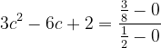
$\dpi{120} 3c^{2}-6c+2=\frac{\frac{3}{8}-0}{\frac{1}{2}-0}$

3c^2-6c+2 = ¾

12c^2- 24c +5 = 0 [multiply both sides with 4]

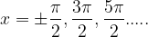
Using quadratic formula to solve this quadratic equation, we get…

$\dpi{120} c=1\pm \left ( \frac{\sqrt{21}}{6} \right )$

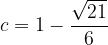
Out of these two values only $\dpi{120} c=1-\frac{\sqrt{21}}{6}$ lies in the given domain.

Hence Mean Value Theorem is verified.

Example 2: A marathoner ran 26 mile, city marathon in 2 hr and 15 min. Like all other runners, he started from a stationary position. During last 5 meters, his leg cramped. He fell down and had to roll across the finish line. Prove that atleast twice, the runner was running at exactly 11 mph.

Solution: Here position function S(t) is a continuous and differentiable function of time t. Which means MVT can be applied here. Since runner start from 0 and stops at finishing line after 2 hours 15 min (2.25 hrs), we have :

$S(0)=0$

$S(2.25)=26$

Average velocity is given as:

$S'(t)=\frac{26-0}{2.25-0}=11.56$

MVT guarantees that runner is running at a speed of 11.56 mph atleast once during his run for 2 hours and 15 min. Since he started at a velocity of 0, reached at a velocity of 11.56 mph and then return back to 0 velocity at finishing line, he must have crossed the velocity of 11mph atleast twivce during his run.

Note: Mean Value Theorem is not applicable to every function.

Here are few examples where MVT is not applicable.

Example 3: Discuss the applicability of Lagrange’s mean value theorem for the following functions.

a) f(x) = |x| on [-1,1]

b) f(x) = 1/x on [-1,1]

Solution:

a) f(x)= |x| is continuous everywhere so it is continuous at [-1,1] . But it is not differentiable on given domain as derivative doesn’t exist at x=0 for f(x)=|x|.

Since second conditions of Mean value theorem is not met , so MVT is not applicable to this function.

b) f(x)= 1/x is not continuous at x=0 which lie on interval [-1,1]. Therefore it is not differentiable at x=0 .

Since both conditions are not met on the given domain so MVT is not applicable to this function on given domain [-1,1]

Practice problems:

Determine all the numbers c which satisfy the conclusions of the Mean Value Theorem for the following function.

$\dpi{120} f(x)=x^{3}+2x^{2}-x$ on [-1,2]

Using mean value theorem, find a point on the curve $\dpi{120} y=\sqrt{x-2}$

defined on the interval [2,3] where the tangent is parallel to the chord joining the end points of the curve.

Answers:

C=0.7863
$\dpi{120} \left ( \frac{9}{4},\frac{1}{2} \right )$

Concavity and Inflection points

October 1, 2019/by admin_ct

Concave up and concave down

When a curve is bent upward like an upright bowl then it is called concave up and when it is bent downward like inverted bowl then it is called concave down as shown below.

The points where the curve changes its concavity are called inflection points. In other words these are the points where curve changes its direction from concave up to concave down and vice versa.

How to find intervals of concavity and inflection points .

Algorithm:

Find derivative f’(x).
Find second derivative f”(x).
Set f”(x)=0 and solve for x to get possible points of inflection.
Using these points find intervals on number line.
Check these intervals one by one using testing points from each interval, plugging them into second derivative f”(x).
If f”(x)> 0 (positive) then function is concave up.
If f”(x)< 0 (negative) then function is concave down.
The points where curve changes its direction are the inflection points.

Example1 : Find intervals when the following function is concave up and down. Also find the points of inflection.

f(x)= x^3 +3x^2 -6x +1

solution:

step 1) f’(x) = 3x^2+6x-6

step 2) f”(x)= 6x+6

step 3) f”(x)=0 => 6x+6 = 0

x= -1

step 4) using x=-1 we get the intervals of concavity on number line as (-∞ ,-1) and (-1,∞ )

step 5) Checking intervals:

for interval (-∞,-1) let x=-2

f”(x) = 6x+6

f”(-2) = 6(-2)+6= -6 < 0 Concave down

for interval (-1,∞ ) let x=0

f”(0) = 6(0)+6 = 6 > 0 Concave up

Step 6) Points of inflection.

We see that concavity changes at x=-1. Graph changes from concave down to concave up at x=-1 so x=-1 is only inflection point.

Note: If (c,f(c)) is an inflection point then either f”(c)=0 or f”(c) is undefined. But not all points where f”(x)=0 or undefined corresponds to inflection points.

Here is an example to show this case.

Example2: Find all the inflection points and intervals of concave up and down for the function

$\dpi{120} {\color{Red} f(x)=(x+1)^{4}}$

Solution: step 1)

$\dpi{120} f'(x)=4(x+1)^{3}$

step 2)

$\dpi{120} f''(x)= 12(x+1)^{2}$

step 3)

$\dpi{120} f''(x)=0\Rightarrow 12(x+1)^{2}=0$

$\dpi{120} (x+1)^{2}=0 \Rightarrow x+1=0$

x = -1 (possible inflection point)

step 4) Using x=-1 we get interval as (-∞,-1) and (-1,∞)

But we observe that f”(x) is positive on both intervals , that means concavity doesn’t change at x=-1, so x=-1 is not an inflection point.

Practice problems:

For the following function, identify the intervals where the function is concave up and concave down. Also find point of inflection.

$\dpi{120} f(x)=3x^{5}-5x^{3}+3$

For the following function find the inflection points and the intervals of concave up/concave down.

$\dpi{120} f(x)=x(6-x)^{\frac{2}{3}}$

Answers:

Concave up : $\dpi{120} \left ( \frac{-1}{\sqrt{2}},0 \right )\cup \left ( \frac{1}{\sqrt{2}},\infty \right )$

Concave down: $\dpi{120} \left (-\infty , \frac{-1}{\sqrt{2}} \right )\cup \left ( 0,\frac{1}{\sqrt{2}}, \right )$

Inflection points: $\dpi{120} x=\frac{-1}{\sqrt{2}},0,\frac{1}{\sqrt{2}}$

Inflection points: x=7.2

Concave down: (0,6)U(6,7.2)

Concave up : (7.2,∞)

Relative(Local) maximum and minimum

October 1, 2019/by admin_ct

How to find Relative maximum and minimum?

An important application of derivatives is, relative(local) maxima and minima. We can find it using two methods as explained below.

Using first derivative test:

Algorithm:

1) Find derivative f ’(x) of given function.

2) Set f ’(x)=0 and solve for x which gives critical numbers.

3) Using these critical numbers find intervals on a number line.

4) Check each interval by taking some testing point from each interval and plugging them into derivative f’(x).

5) If we get f ’(c)>0(positive) then function is increasing on that interval.

If f ’(x)<0(negative) then function is decreasing on that interval.

6) The point when derivative changes from negative to positive is called relative minima.

The point when derivative changes from positive to negative is called relative maxima.

Example1 : Find all the points of relative maxima and minima of given function

${\color{Red} f(x)=x^3-6x^2+9x-8}$

Solution :

Step 1) $f'(x)=3x^2 -12x+9$

Step 2) $f'(x)=0$

$3x^2 -12x+9 =0$

$3(x^2 -4x+3)=0$

$3(x-3)(x-1)=0$

$(x-3)=0 , (x-1)=0$

$x=3, x=1$

Critical numbers : x=3,1

Step 3) Using these critical numbers on number line, we find intervals as (-∞,1) ,(1,3), (3,∞)

Step 4) Checking intervals :

For interval (-∞,1) let x=0

$f'(0)= 3(0)^2-12(0)+9 =9 >0$ Increasing

For interval (1,3) let x=2

$f'(2)= 3(2)^2-12(2)+9 = -3 < 0$ decreasing

For interval (3,∞) let x=4

$f'(4)= 3(4)^2-12(4)+9 =9 >0$ Increasing

Step 5) Since derivative changes from + to – at point x=1 so x=1 is relative (local) maximum.

Since derivative changes from – to + at x=3 so x=3 is relative (local) minimum..

Using second derivative method:

Initial steps are same as used for first derivative test.

1) Find derivative f ’(x) .

2) Set derivative f’(x)=0 and find critical numbers.

3) Find second derivative f”(x)

4) Plugin critical numbers into second derivative f”(x) one by one.

5) If f”(c) > 0 then point c is relative minima.

If f”(c) < 0 the point c is relative maxima.

Now we are going to solve same problem using second derivative test and see if we get same answer.

Example : ${\color{Red} f(x)=x^3-6x^2+9x-8}$

Step 1)

$f'(x)=3x^2 -12x+9$

Step 2) $f'(x)=0$

$3x^2 -12x+9 =0$

$3(x^2 -4x+3)=0$

$3(x-3)(x-1)=0$

$(x-3)=0 , (x-1)=0$

$x=3, x=1$

Step 3)

$f''(x) = 6x-12$

Step4)

$f''(1) = 6(1)-12 =-6 < 0$ Relative maximum

$f''(3) = 6(3)-12 =6 > 0$ Relative minimum

Note: Second derivative test method is easier and shorter to find relative maxima and minima but sometimes it is hard to find second derivative then it is wiser to use first derivative test.

Example : Find the values of a,b and c so that graph of ${\color{Red} y=\frac{x^2+a}{bx+c}}$ has local minimum at x=3 and local maximum at (-1,-2).

Here is the solution in this video.

Critical numbers and some special cases:

What is critical number?

A number c in the domain of f(x) is called critical number of f(x) if f ‘(c) =0 or f ‘(c) is undefined.

Using Fermat theorem, if f(c) is local maximum or minimum then c must be a critical number. That means local maxima or minima can occur only at critical numbers but not every critical number is local extremum.

This can be illustrated in following examples.

Example3: Find critical numbers and local extrema of

${\color{Red} f(x)=x^3}$

Solution:

$f'(x)= 3x^2$

$f'(x) =0$

$3x^2= 0$

$x^2 =0$

$x=0$

x=0 is the only critical number here.

But x=0 is not a local maximum or minimum as derivative doesn’t change its sign at x=0

Example4: Find critical numbers and local extrema of

${\color{Red} f(x) =x^{\frac{1}{3}}}$

Solution:

$\dpi{120} f(x)=x^{\frac{1}{3}}$

$\dpi{120} f'(x)=\frac{1}{3}x^{\frac{-2}{3}} = \frac{1}{3x^{\frac{2}{3}}}$

$\dpi{120} f'(x)=0 \Rightarrow \frac{1}{3x^{\frac{2}{3}}}=0$

We see that x=0 is critical number here as derivative is not defined at x=0, but this critical number is not a local maximum or minimum as derivative doesn’t change its sign at 0.

Practice problems:

Find all the points of relative(local) maxima and minima and the corresponding maximum and minimum values of the function.

$\dpi{120} f(x)= 2x^{3}-21x^{2}+36x-20$

Find the points of relative(local) maxima and minima and the corresponding maximum and minimum values of the function.

f(x)= sin(2x) –x where $\frac{-\pi }{2}\leq x\leq \frac{\pi }{2}$

Write all answers in ordered pair

Answers:

Local maximum (1,-3)

Local minimum (6,-128)

Local maximum $\dpi{100} \left ( \frac{\pi }{6} ,\frac{\sqrt{3}}{2}-\frac{\pi }{6}\right )$

Local minimum $\dpi{100} \left ( \frac{-\pi }{6} ,\frac{-\sqrt{3}}{2}+\frac{\pi }{6}\right )$

Understanding difference between Relative and Absolute extrema

October 1, 2019/by admin_ct

Maxima and Minima : Differentiation is used to find maximum and minimum values of differentiable functions in their domains. There are two types of extrema(maxima & minima).

Relative (local) extrema: These are the turning points in the domain of function at which function has a value which is greater (for maxima) or smaller (for minima) than the values at its neighbouring points. There can be more than one relative maxima or minima for a function.

Absolute extrema: These extreme values are found on a closed interval. Absolute maxima is the greatest value of the continuous function for given closed interval and absolute minima is the smallest value of continuous function on given closed interval. It may be at critical points or at the end points of given closed interval. There can be only one absolute maximum and minimum value for the given domain.

Difference between Relative and Absolute extrema.

Difference between two types of extrema can be understood with a beautiful example here.

Assume a country having many states. Each state has an airport which serves domestic interstate flights. All these state airports are local (relative) extrema. But There is an international airport in the capital city which serves international flights connecting to other countries. This international airport is absolute extrema. There can be more than one one local maxima and minima(like many state airports) but there is only one absolute maxima and minima like international airport in capital city.

Absolute maxima and minima

September 30, 2019/by admin_ct

How to find Absolute maxima/minima on a closed interval.

When we study maximum and minimum values on a closed interval [a,b] for a continuous function f(x) then it is called absolute maxima/minima. We study values at end points of this closed interval as well as critical points which lie inside this closed interval. We are not concerned critical points which lie outside the given closed interval.

To find absolute maxima/minima, we use following procedure .

Algorithm:

Find derivative f’(x).
Set f’(x)=0 and solve for x to get critical numbers.
Choose the critical numbers which lie on given closed interval.
Plug in all the valid critical numbers as well as end points of given closed interval into original function.
The greatest value among all these values is absolute maxima and the smallest value among all these values is absolute minima.

Example 1: Find absolute maxima and minima for given function on closed interval [1,3]

${\color{Red} f(x)= 2x^3 -24x +107}$

solution:

step 1) $f'(x) = 6x^2 -14$

step2) $f'(x) =0$

$6x^2 -24 =0$

$6(x^2 -4)=0$

$x^2 -4 =0$

$x= -2, 2$

Out of these two critical points only x=2 is applicable as it lies on the given interval [1,3]. Now we check value of function at critical point x=2 as well as end points x=1 and x=3.

$f(x)= 2x^3-24x+107$

$f(1)= 2(1)^3 -24(1)+107 = 85$

$f(2)= 2(2)^3 -24(2)+107 = 75$

$f(3)= 2(3)^3 -24(3)+107 = 89$

Out of these values 89 is the greatest and 75 is the smallest. So x=3 is absolute maxima and x=2 is absolute minima and we can write absolute maximum and minimum values as ordered pair.

Absolute maxima = (3,89)

Absolute minima = (2,75)

Question: Does every function has an absolute maximum and an absolute minimum ?

Answer: No, Not every function has absolute maxima and minima. Only a continuous function defined on a closed interval can have absolute maximum and minimum.

Here is an example to understand the difference.

Example2: Locate any absolute extrema of function

${\color{Red} f(x)= x^2 -9}$

a) on the open interval (-∞,∞)

b) on the open interval (-3,3)

c) on the closed interval [-3,3]

Solution: Lets look at graphs of function in all three cases.

We can see that both ends of graph are approaching to infinity, so it has no absolute maximum value but it has absolute minimum value at vertex (0,-9).

Absolute maximum : None

Absolute minimum : f(0) = -9 , (0,-9)

By looking at first graph, we may think it has absolute maxima at x=0 but it is not the case. Since this is an open interval so end points can’t be considered. This one too has absolute minimum as f(0)=-9 but no absolute maximum.

Absolute maximum : None

Absolute minimum : f(0) = -9

(0,-9)

c) In this case, end points -3 and 3 are considered because of closed interval. So this graph has absolute maximum values at end points f(-3)=f(3)=0.

Absolute maximum : f(-3) = f(3) = 0

(-3,0) and (3,0)

Absolute minimum : f(0) = -9

(0,-9)

Example3: Find absolute maximum and absolute minimum of ${\color{Red} f(x)= \frac{1}{x}}$ on interval [-3,0)U(0,3]

Solution: As this function is not continuous throughout the interval [-3,3], it fails to have any absolute maximum and minimum.

Here we make use of the following extreme value theorem:

A continuous function defined on a closed , bounded interval [a,b] attains both an absolute maximum and minimum on that inertval.

Practice problems:

Find absolute maximum and minimum values for the following functions in the given intervals.

$\dpi{120} f(x)= 3x^{4}-8x^{3}+12x^{2}-48x+1$ on [ 1,4 ]

Find absolute maximum and minimum values of

f(x)=x+sin(2x) on [0,2π]

Answers:

Absolute maximum (4,257)

Absolute minimum (2,-59)

Absolute maximum (2π,2π)

Absolute minimum (0,0)

Logarithmic Differentiation

September 29, 2019/by admin_ct

Derivative using Logarithmic differentiation.

So far we have discussed derivatives of the functions of the form $\dpi{120} \left ( f(x) \right )^{n}$ where f(x) is a function of x and n is constant. But when we are given functions of the form $\dpi{120} f(x)^{g(x)}$ where no other ordinary rules apply, then we use logarithmic differentiation. To find derivative of such type of functions, we proceed as follows.

Let y = $\dpi{120} f(x)^{g(x)}$

Step 1) Taking log of both sides, we get

Log y = log $\dpi{120} f(x)^{g(x)}$

Log y = g(x) log f(x)

Step 2) Differentiating both sides with respect to x,

y’/y = g(x) [log f(x)]’ +g’(x) log f(x) [used product rule here]

$\dpi{120} \frac{y'}{y}= g(x)\frac{f'(x)}{f(x)}+g'(x)log f(x)$

Step 3) $\dpi{120} \frac{y'}{y}= g(x)\frac{f'(x)}{f(x)}+g'(x)log f(x)$ [multiply both sides with y]

$\dpi{120} y' = y [g(x)\frac{f'(x)}{f(x)}+g'(x)log f(x)]$

$\dpi{120} y' = f(x)^{g(x)} [g(x)\frac{f'(x)}{f(x)}+g'(x)log f(x)]$

Lets work on some examples to understand this process better.

Example1 : Find derivative of $\dpi{120} {\color{Red} y= x^{sinx}}$

Solution: Here the base(x) and power (sinx) of this expression, both are functions of x so we use logarithmic differentiation.

Using the same process as given above we move as follows :

Step 1) Taking log of both sides

$\dpi{120} logy =log\left ( x^{sinx} \right )$

Log y = sinx logx

Step2) Differentiating both sides with respect to x,

(logy)’= [(sinx)’logx+sinx(logx)’] [used product rule]

$\dpi{120} \frac{y'}{y}=cosx logx+\frac{sinx}{x}$

step 3) Multiply both sides with y,

$\dpi{120} y' = y \left [cosx logx+\frac{sinx}{x} \right ]$

$\dpi{120} y' = x^{sinx} \left [cosx logx+\frac{sinx}{x} \right ]$ [answer]

Logarithmic differentiation is also used to differentiate complex algebraic functions in an efficient manner, where otherwise you have to use product rule, quotient rule and chain rule altogether and do some messy calculations. Here is such an example .

Example2: Find the derivative of $\dpi{120} {\color{Red} y=\frac{x^{3}(x^{2}+1)^{4}}{\sqrt[3]{3x+2}}}$

Solution: This derivative can be found using quotient rule , power rule and chain rule but instead of using all these rules we can use just logarithmic differentiation and avoid messy calculations.

Step 1) Taking log of both sides…

$\dpi{120} log(y)=log\left [\frac{x^{3}(x^{2}+1)^{4}}{\sqrt[3]{3x+2}} \right ]$

Simplify using properties of log,

$\dpi{120} logy = log(x^{3})+log(x^{2}+1)^{4}-log(\sqrt[3]{3x+2})$

$\dpi{120} logy = 3log(x)+4log(x^{2}+1)-log(3x+2)^{\frac{1}{3}}$

$\dpi{120} logy = 3log(x)+4log(x^{2}+1)-\frac{1}{3}log(3x+2)$

Step 2) Differentiating both sides with respect to x,

$\dpi{120} (logy)' = 3(log(x))'+4(log(x^{2}+1))'-\frac{1}{3}(log(3x+2))'$

$\dpi{120} \frac{y'}{y} = 3\left (\frac{1}{x} \right )+4\left ( \frac{2x}{x^{2}+1} \right )-\frac{1}{3}*\frac{3}{3x+2}$

$\dpi{120} \frac{y'}{y} = \left (\frac{3}{x} \right )+\left ( \frac{8x}{x^{2}+1} \right )-\frac{1}{3x+2}$

Step 3) Multiply both sides with y,

$\dpi{120} y' = y \left [\left (\frac{3}{x} \right )+\left ( \frac{8x}{x^{2}+1} \right )-\frac{1}{3x+2} \right ]$

$\dpi{120} y' = \frac{x^{3}(x^{2}+1)^{4}}{\sqrt[3]{3x+2}} \left [\left (\frac{3}{x} \right )+\left ( \frac{8x}{x^{2}+1} \right )-\frac{1}{3x+2} \right ]$ [ answer]

Example3: If $\dpi{120} {\color{Red} x^{m}y^{n}=(x+y)^{m+n}}$ prove that $\dpi{120} {\color{Red} \frac{\mathrm{d} y}{\mathrm{d} x}=\frac{y}{x}}$ and then $\dpi{120} {\color{Red} \frac{\mathrm{d}^{2}y }{\mathrm{d} x^{2}}=0}$

Solution: $\dpi{120} x^{m}y^{n}=(x+y)^{m+n}$

Step1 ) Taking log of both sides ,

$\dpi{120} \log \left (x^{m}y^{n} \right )=\log(x+y)^{m+n}$

$\dpi{120} logx^{m}+logx^{n}=(m+n) log(x+y)$

m logx + n logy = (m+n) log(x+y)

Step2) Taking derivative of both sides with respect to x,

$\dpi{120} \frac{m}{x}+\frac{n}{y}y'= (m+n)\frac{1+y'}{x+y}$

$\dpi{120} \frac{m}{x}+\frac{n}{y}y'= (m+n)\left ( \frac{1}{x+y}+\frac{y'}{x+y}\right )$

$\dpi{120} \frac{m}{x}+\frac{n}{y}y'= \frac{m+n}{x+y}+\frac{(m+n)y'}{x+y}$

$\dpi{120} \frac{n}{y}y'-\frac{(m+n)y'}{x+y}= \frac{m+n}{x+y}-\frac{m}{x}$

$\dpi{120} \left (\frac{n}{y}-\frac{(m+n)}{x+y} \right )y'= \frac{x(m+n)-m(x+y)}{x(x+y)}$

$\dpi{120} \left (\frac{n(x+y)-y(m+n)}{y(x+y)} \right )y'= \frac{mx+nx-mx-my}{x(x+y)}$

$\dpi{120} \left (\frac{nx+ny-my-ny}{y(x+y)} \right )y'= \frac{nx-my}{x(x+y)}$

$\dpi{120} \left (\frac{nx-my}{y(x+y)} \right )y'= \frac{nx-my}{x(x+y)}$

$\dpi{120} y'= \frac{nx-my}{x(x+y)}*\frac{y(x+y)}{nx-my}=\frac{y}{x}$

$\dpi{120} y'= yx^{-1}$

$\dpi{120} y''= y(x^{-1})'+(y)'(x^{-1})$ [used product rule]

$\dpi{120} y''= y(-1*x^{-2})+y'(x^{-1})$

$\dpi{120} y''= \frac{-y}{x^{2}}+\frac{y'}{x}$

$\dpi{120} y''= \frac{-y}{x^{2}}+\frac{\frac{y}{x}}{x}$

$\dpi{120} y''= \frac{-y}{x^{2}}+\frac{y}{x^{2}}=0$ [answer]

Practice problems:

Find derivative of following using logarithmic differentiation:

$\dpi{120} y=sinx^{tanx}$
$\dpi{120} y=x^{\sqrt{x}}$
$\dpi{120} y=\frac{\sqrt{1-x^{2}}(2x-3)^{\frac{1}{2}}}{(x^{2}+2)\frac{2}{3}}$
$\dpi{120} y=\sqrt{\frac{1+x}{1-x}}$

Answers:

$\dpi{120} sinx^{tanx}\left [ sec^{2}x log(sinx) +1\right ]$
$\dpi{120} x^{\sqrt{x}}\left [ \frac{logx}{2\sqrt{x}}+\frac{1}{\sqrt{x}} \right ]$
$\dpi{120} \frac{\sqrt{1-x^{2}}(2x-3)^{\frac{1}{2}}}{(x^{2}+2)\frac{2}{3}}\left [ \frac{-x}{(1-x^{2})} +\frac{1}{2x-3}-\frac{4x}{3(x^{2}+2)}\right ]$
$\dpi{120} \sqrt{\frac{1+x}{1-x}}\left [ \frac{1}{(1-x^{2})} \right ]$

Implicit Differentiation

September 29, 2019/by admin_ct

How to find derivatives of Implicit functions

So far we have discussed derivatives of the functions of the form y=f(x). This is called explicit form but some relationships can’t be represented by an explicit function.

If the variables x and y are connected by a relation f(x,y)=0 and it is not possible or convenient to express y as a function of x, then y is said to be an implicit function of x. In such case we differentiate both sides of given relation with respect to x to isolate dy/dx at the end. Such type of differentiation is called implicit differentiation. Lets look into some examples:

For the sake of simplicity lets use y’ instead of dy/dx for all problems of implicit differentiation.

Example1: Find y’ if (x+y)sin(xy)=x^2

Solution: (x+y) sin(xy)= x^2

(1+y’)sin(xy)+(x+y)cos(xy)(y+xy’)=2x [used product rule and chain rule]

sin(xy)+y’sin(xy) + (x+y)cos(xy)y +(x+y)cos(xy)xy’ =2x

y’sin(xy) +(x+y)cos(xy) xy’ =2x-sin(xy) –(x+y)cos(xy)y

y’[sin(xy)+(x+y)cos(xy)x] = 2x-sin(xy) –(x+y)cos(xy)y

$\dpi{120} y' =\frac{2x-sin(xy)-(x+y)cos(xy)y}{sin(xy)+(x+y)cos(xy)x}$ [answer]

Example 2 : Find second derivative of the function $\dpi{120} {\color{Red} y^{5}+x^{5}=10}$

solution: Taking derivative of both sides with respect to x,

$\dpi{120} 5y^{4}y'+5x^{4}=0$

$\dpi{120} 5y^{4}y'=- 5x^{4}$

$\dpi{120} y^{4}y'=- x^{4}$

$\dpi{120} y' = \frac{-x^{4}}{y^{4}}$ [First derivative]

Differentiating $\dpi{120} y^{4}y'=- x^{4}$ again with respect to x,

$\dpi{120} [(y^{4})'y'+y^{4}y'']=-4x^{3}$ [ used product rule on left side]

$\dpi{120} [4y^{3}y'y'+y^{4}y'']=-4x^{3}$

$\dpi{120} y^{4}y''=-4x^{3}-4y^{3}y' y'$

$\dpi{120} y^{4}y''=-4x^{3}-4y^{3}(y')^{2}$

$\dpi{120} y^{4}y''=-4x^{3}-4y^{3}(\frac{-x^{4}}{y^{4}})^{2}$

$\dpi{120} y^{4}y''=-4x^{3}-4y^{3}\frac{x^{8}}{y^{8}}$

$\dpi{120} y^{4}y''=-4x^{3}-\frac{4x^{8}}{y^{5}}$

Multiplying both sides with y^5 we get,

$\dpi{120} y^{9}y''=-4x^{3}y^{5}+4x^{8}$

$\dpi{120} y'' = \frac{-4x^{3}y^{5}+4x^{8}}{y^{9}}$ [ answer]

Example 3: Find the slope of tangent line to the curve y+xcosy=cosx at point (0,1)

Solution: y+xcosy = cosx

Differentiating both sides with respect to x,

Y’ + [(x)’cosy +x(cosy)’] = -sinx

Y’ +[1*cosy +x(-siny)y’] = -sinx

Y’ + cosy-xsiny y’ = -sinx

Y’- x siny y’ = -sinx –cosy

Y’(1-x siny) = -sinx –cosy

$\dpi{120} y' =\frac{-sinx-cosy}{1-xsiny}$

Now plugin given point x=0 , y=1 into derivative expression.

$\dpi{120} y' =\frac{-sin(0)-cos(1)}{1-(0)sin(1)}$

$\dpi{120} y' =\frac{0-cos(1)}{1-0}$

Y’ = -cos(1) [answer]

Example4: Use implicit differentiation, find the points where graph of given equation has horizontal tangents .

$\dpi{120} {\color{Red} 2x^{2}+y^{2}-4x+2y+2 =0}$

Solution: Differentiating given equation with respect to x,

2(x^2 )’ +( y^2)’ -4x’+2y’ +2’=0

2(2x) +2yy’ -4(1) +2y’ +0 =0

4x + 2yy’ -4 +2y’ =0

2y’(y+1) = 4-4x

$\dpi{120} y'=\frac{4(1-x)}{2(y+1)}=\frac{2(1-x)}{y+1}$

For horizontal tangents , slope is 0 , therefore

Y’ =0

Which implies:

$\dpi{120} \frac{2(1-x)}{y+1}=0$

2(1-x)=0

1= x

To find y values at x=1 we plugin into original equation,

$\dpi{120} 2(1)^{2}+y^{2}-4(1)+2y+2 =0$

$\dpi{120} 2+y^{2}-4+2y+2 =0$

$\dpi{120} y^{2}+2y =0$

y(y+2) =0

y=0 , y=-2

So the points of horizontal tangents are: (1,0) and (1,-2)

To find vertical tangents we set denominator of derivative =0 and solve to get points same way.

Practice problems:

Find derivative of following implicit functions.

1. $\dpi{120} \sqrt{x}+\sqrt{y}=1$

2. $\dpi{120} 2x^{3}=(3xy+1)^{2}$

Find y’’ for the following function.

3. $\dpi{120} 3x^{2}+2y^{2}=12$

Find slope of curve at given point.

4. $\dpi{120} xy^{5}+x^{5}y=1$ at point (-1,-1)

Answers:

$\dpi{120} \frac{-\sqrt{y}}{\sqrt{x}}$
$\dpi{120} \frac{-3y^{2}x-y+x^{2}}{3x^{2}y+x}$
$\dpi{120} \frac{-9}{y^{3}}$
slope = -1

The Quotient rule of Derivatives

September 28, 2019/by admin_ct

Derivative Using Quotient rule

This rule is used to find derivative of rational functions which are the ratio of two algebraic expressions. Lets assume two algebraic expressions f(x) as numerator and g(x) as denominator such that both functions are differentiable and g(x)≠0 , then quotient rule is defined as…..

$\dpi{150} \mathbf{\left [ \frac{f(x)}{g(x)} \right ]'=\frac{g(x)f'(x)-f(x)g'(x)}{[g(x)]^{2}}}$

Lets work on some example to understand this rule.

Example1: Find derivative of $\dpi{120} {\color{Red} y=\frac{2x-3}{x+1}}$

Solution: Lets assume f(x)= 2x-3 g(x)= x+1

f’(x) =2 g’(x)= 1

Substituting these values into the quotient rule we get,

$\dpi{120} \left [ \frac{f(x)}{g(x)} \right ]'=\frac{g(x)f'(x)-f(x)g'(x)}{[g(x)]^{2}}$

$\dpi{120} Y'=\frac{(x+1)(2)-(2x-3)(1)}{(x+1)^{2}}$

$\dpi{120} Y'=\frac{2x+2-2x+3}{(x+1)^{2}}$

$\dpi{120} Y'=\frac{5x}{(x+1)^{2}}$ [Answer]

Example2: Find derivative of $\dpi{120} {\color{Red} y=\frac{sinx+cosx}{sinx-cosx}}$

Solution: let

f(x) = sinx+cosx g(x) = sinx-cosx

f ’(x) = cosx-sinx g’(x) = cosx+sinx

$\dpi{120} \left [ \frac{f(x)}{g(x)} \right ]'=\frac{g(x)f'(x)-f(x)g'(x)}{[g(x)]^{2}}$

$\dpi{120} Y'=\frac{(sinx-cosx)(cosx-sinx)-(sinx+cosx)(cosx+sinx)}{[sinx-cosx]^{2}}$

$\dpi{120} Y'=\frac{2sinxcosx-sin^{2}x-cos^{2}x-2sinxcosx-sin^{2}x-cos^{2}x}{[sinx-cosx]^{2}}$

$\dpi{120} Y'=\frac{-2sin^{2}x-2cos^{2}x}{sin^{2}x+cos^{2}x-2sinxcosx}$

$\dpi{120} Y'=\frac{-2(sin^{2}x+cos^{2}x)}{1-2sinxcosx}$

$\dpi{120} Y'=\frac{-2(1)}{1-sin2x}$

$\dpi{120} Y'=\frac{-2}{1-sin2x}$

Different ways to find derivative of rational function.

In addition to quotient rule, derivative of rational functions can also be found using other ways. Sometimes these ways proved to be easier and shorter. Product rule can also be used to find derivative of rational function.Here are few examples in this vedio.